User:Captain Blood~enwiki/GMT Example


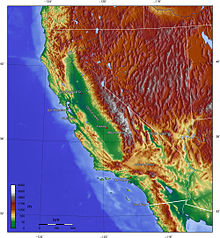
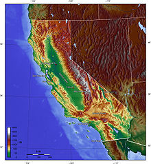
How to create a topographic map with GMT
[edit]Here is described how one can create a map of California.
Installation
[edit]Install the Generic Mapping Tools (must use Version 4.X+), Linux is preferred (Windows is possible too, but I don't know about that (NOTE: Tested in Windows. Use the script in a Cygwin shell (to eliminate rewrite))). Either way Ghostscript or other PostScript software is needed too. Read GMT's tutorial [1]. Especially sections 4.1.3, 4.1.4 (how to create simple maps) and 4.3 (using grid files for the relief). Anyway, be aware GMT is a set of command line tools, there is no GUI. There exists a GUI frontend for GMT, see the external link in Generic Mapping Tools but I haven't tried that.
Topographic data
[edit]Download e10g.tgz from http://www.ngdc.noaa.gov/mgg/topo/gltiles.html and untar it into GMTHOME/GMT4.0/share/dbase
If you want bathymetry (oceanic topography), download etopo2.grd from http://rda.ucar.edu/datasets/ds759.3/ (registration required, free). It is already in GMT's grd-format.
NOTE:Despite the similarity of names, the etopo2.grd file covers the entire world, while e10g only covers a western portion of North America.
Gridfiles
[edit]Add the following lines into GMTHOME/GMT4.0/share/dbase/grdraster.info (we need line 5 only now, but the other may become useful)
  1 "GLOBE_G" "m" -R-180/-90/50/90 -I0.5m P i 1 0 -500 a10g
  2 "GLOBE_G" "m" -R-90/0/50/90    -I0.5m P i 1 0 -500 b10g
  3 "GLOBE_G" "m" -R0/90/50/90     -I0.5m P i 1 0 -500 c10g
  4 "GLOBE_G" "m" -R90/180/50/90   -I0.5m P i 1 0 -500 d10g

  5 "GLOBE_G" "m" -R-180/-90/0/50  -I0.5m P i 1 0 -500 e10g
  6 "GLOBE_G" "m" -R-90/0/0/50     -I0.5m P i 1 0 -500 f10g
  7 "GLOBE_G" "m" -R0/90/0/50      -I0.5m P i 1 0 -500 g10g
  8 "GLOBE_G" "m" -R90/180/0/50    -I0.5m P i 1 0 -500 h10g

  9  "GLOBE_G" "m" -R-180/-90/-50/0 -I0.5m P i 1 0 -500 i10g
  10 "GLOBE_G" "m" -R-90/0/-50/0    -I0.5m P i 1 0 -500 j10g
  11 "GLOBE_G" "m" -R0/90/-50/0     -I0.5m P i 1 0 -500 k10g
  12 "GLOBE_G" "m" -R90/180/-50/0   -I0.5m P i 1 0 -500 l10g

  13 "GLOBE_G" "m" -R-180/-90/-90/-50  -I0.5m P i 1 0 -500 m10g
  14 "GLOBE_G" "m" -R-90/0/-90/-50     -I0.5m P i 1 0 -500 n10g
  15 "GLOBE_G" "m" -R0/90/-90/-50      -I0.5m P i 1 0 -500 o10g
  16 "GLOBE_G" "m" -R90/180/-90/-50    -I0.5m P i 1 0 -500 p10g
NOTE:  Although this article was originally written with blank lines between some of
 the text lines (ex. lines 4 and 5, lines 8 and 9), the grdraster.info file MUST NOT
 have blank lines before, in between, or after the lines with text. Otherwise, you will
 receive an error "ERROR reading grdraster.info file." "File number conversion error."
FURTHER NOTE:  At least in Windows, there must be a carriage return/line feed (CRLF)
 at the end of the last line or the p10g file will not be processed.
Create the gridfile e.grd (from anywhere) (see GMT tutorial chapter 4.3):
grdraster 5 -R-180/-90/0/50 -Ge.grd
Create the illuminated gridfile e_i5.grd:
grdgradient e.grd -Ne.5 -A100 -M -Ge_i5.grd
Labels
[edit]The following textfiles contain some labels and coordinates:
  # file california_capital
  -121:29 38:34 10 0 0 BR SACRAMENTO
  # file california_cities
  -118:14 34:03 10 0 0 TR Los Angeles
  -122:25 37:46 10 0 0 TR San Francisco
  -121:53 37:20 10 0 0 TR San Jose
  -119:46 36:44 10 0 0 BR Fresno
  -117:09 32:42 10 0 0 TR San Diego
  # file california_cross
  -117:00 36:30 10 0 2 TL Death Valley
  # file california_labels
  12 15 10 -55 2 MC Sierra Nevada
  10 14 10 -50 2 MC Central Valley
  16  8 10   0 2 MC Mojave Desert
  # file california_peaks
  -118:17:31 36:34:43 10 0 2 TR Mount Whitney
Color palettes
[edit]The color palette for the topography:
  # file usa.cpt
  #COLOR_MODEL = RGB
  #
  0	0	97	71	50	16	122	47
  50	16	122	47	500	232	215	125
  500	232	215	125	1200	161	67	0
  1200	161	67	0	1700	130	30	30
  1700	130	30	30	2800	110	110	110
  2800	110	110	110	4000	255	255	255
  4000	255	255	255	6000	255	255	255
  N 0 97 71
  F 255 0 0
  B 0 97 71
The color palette for the bathymetry (optional)
  # file meer.cpt
  #COLOR_MODEL = RGB
  #
  -11000   36  38 175     -5500   56  58 195
  -5500	 56  58 195	-3000	70  72 214
  -3000	 70  72 214	-2000	81 102 217
  -2000	 81 102 217	 -750	100 129 223
   -750	100 129 223	  -70	131 161 230
    -70	131 161 230	  -20	164 192 240
    -20	164 192 240	    0	170 200 255
  N 170 200 255
  F 170 200 255
  B 170 200 255
The Map
[edit]Not the final step, but the most important: run the following shell script:
   #!/bin/bash

   FILE=california
   AREA=-R-126/31/-112/43r
   PROJ=-JB-120.5/37/33/41/24c
   DETAIL=-Dh
   GRID=4
   SCALE=-Lf-123/31.55/37/200k
   NATION1=-N1/8/255/255/255
   NATION2=-N2/3/255/255/255
   LAND=-G155/155/155
   WATER=-S150/150/255
   COAST=-W2/40/40/120
   RIVERS="-Ia/1/40/40/120 -I1/4/40/40/120 -I2/2/40/40/120"
   ALL="-P $AREA $PROJ"
   TOPO=e.grd
   ILLU=-Ie_i5.grd
   PALETTE=-Cusa.cpt
   TOPO2=etopo2.grd
   PALETTE2=-Cmeer.cpt

   # TOPO ########################################################################
   # bathymetry
   grdimage $TOPO2 $PALETTE2 $ALL -K >temp.ps
   # clippath for land
   pscoast $ALL $DETAIL -Gc -K -O >>temp.ps
   # land
   grdimage $TOPO $ILLU $PALETTE $ALL -K -O >>temp.ps
   # clear clippath
   pscoast -R -J -O -K -Q >>temp.ps

   cp temp.ps topo.ps

   # coast, rivers
   pscoast $ALL $DETAIL -B"$GRID"g"$GRID" $COAST $RIVERS $NATION1 $NATION2 \
    $SCALE -O -K >>topo.ps
   psscale -D.4c/3.0c/2i/.2i $PALETTE -B:m: -L -P -O -K >>topo.ps

   # NATION ######################################################################
   pscoast $ALL $LAND $WATER $DETAIL $LAND $NATION1 $NATION2 -B"$GRID"g0 \
       >nation.ps

   # LABELS ######################################################################
   function do_text ()
       # $1: Koordinaten-Datei
       # $2: Textfarbe ("-G0/0/0 -W178/93/155")
       # $3: Symbol+Farbe ("-Sc.045 -G255/0/0 -W")
       # $4: ps Datei
   {
       # echo "do_text($*)"
       # BL/BR/TR/TL rausfiltern, Labels drucken
       grep BL $1 | pstext $ALL $2 -D.07/.07   -O -K >>$4
       grep BR $1 | pstext $ALL $2 -D-.14/.07  -O -K >>$4
       grep TR $1 | pstext $ALL $2 -D-.14/-.04 -O -K >>$4
       grep TL $1 | pstext $ALL $2 -D.07/-.04  -O -K >>$4
       grep BC $1 | pstext $ALL $2 -D0.0/.07   -O -K >>$4
       grep TC $1 | pstext $ALL $2 -D0.0/-.07  -O -K >>$4
       # Symbole drucken
       psxy $1 $ALL $3 -O -K >>$4
   }

   TF=topo.ps
   TEXTF="-G255/255/255 -S4/0/0/0"
   SYMBF="-G255/0/0 -W2/0/0/0"
   do_text "$FILE"_cities "$TEXTF" "-Ss.2 $SYMBF" $TF
   do_text "$FILE"_capital "$TEXTF" "-Sa.3 $SYMBF" $TF
   do_text "$FILE"_peaks "$TEXTF" "-St.25 -W3/0/0/0" $TF
   do_text "$FILE"_cross "$TEXTF" "-Sx.25 -W3/0/0/0" $TF
   # GRID2=-B1g1
   pstext "$FILE"_labels $GRID2 -JX24c/27c -R0/24/0/27 $TEXTF -O >>$TF
This will create the PostScript files topo.ps and nation.ps.
The final map
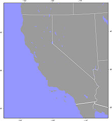
[edit]Open topo.ps and nation.ps with GIMP (300 Dpi), topo.ps with anti-aliasing, nation.ps without. Crop them. Add a layer to topo.ps, copy nation.ps into the new layer, fill all gray areas with black, remove everything else, put the transparency of the new layer at 40%. All land is darker now. Mark california with the color selection tool and cut it. It is bright now. Scale down to 1400 pixels. That's all!
