Deep backward stochastic differential equation method

Deep backward stochastic differential equation method is a numerical method that combines deep learning with Backward stochastic differential equation (BSDE). This method is particularly useful for solving high-dimensional problems in financial derivatives pricing and risk management. By leveraging the powerful function approximation capabilities of deep neural networks, deep BSDE addresses the computational challenges faced by traditional numerical methods in high-dimensional settings.[1]
History
[edit]Backwards stochastic differential equations
[edit]BSDEs were first introduced by Pardoux and Peng in 1990 and have since become essential tools in stochastic control and financial mathematics. In the 1990s, Étienne Pardoux and Shige Peng established the existence and uniqueness theory for BSDE solutions, applying BSDEs to financial mathematics and control theory. For instance, BSDEs have been widely used in option pricing, risk measurement, and dynamic hedging.[2]
Deep learning
[edit]Deep Learning is a machine learning method based on multilayer neural networks. Its core concept can be traced back to the neural computing models of the 1940s. In the 1980s, the proposal of the backpropagation algorithm made the training of multilayer neural networks possible. In 2006, the Deep Belief Networks proposed by Geoffrey Hinton and others rekindled interest in deep learning. Since then, deep learning has made groundbreaking advancements in image processing, speech recognition, natural language processing, and other fields.[3]
Limitations of traditional numerical methods
[edit]Traditional numerical methods for solving stochastic differential equations[4] include the Euler–Maruyama method, Milstein method, Runge–Kutta method (SDE) and methods based on different representations of iterated stochastic integrals.[5][6]
But as financial problems become more complex, traditional numerical methods for BSDEs (such as the Monte Carlo method, finite difference method, etc.) have shown limitations such as high computational complexity and the curse of dimensionality.[1]
- In high-dimensional scenarios, the Monte Carlo method requires numerous simulation paths to ensure accuracy, resulting in lengthy computation times. In particular, for nonlinear BSDEs, the convergence rate is slow, making it challenging to handle complex financial derivative pricing problems.[7][8]

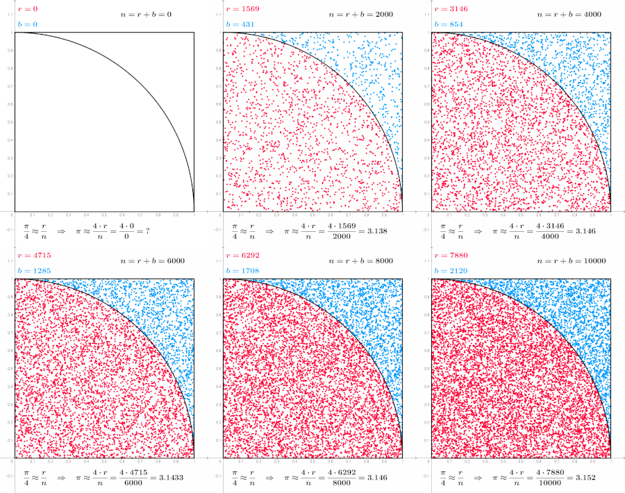
Monte Carlo method applied to approximating the value of π - The finite difference method, on the other hand, experiences exponential growth in the number of computation grids with increasing dimensions, leading to significant computational and storage demands. This method is generally suitable for simple boundary conditions and low-dimensional BSDEs, but it is less effective in complex situations.[9]
Deep BSDE method
[edit]The combination of deep learning with BSDEs, known as deep BSDE, was proposed by Han, Jentzen, and E in 2018 as a solution to the high-dimensional challenges faced by traditional numerical methods. The Deep BSDE approach leverages the powerful nonlinear fitting capabilities of deep learning, approximating the solution of BSDEs by constructing neural networks. The specific idea is to represent the solution of a BSDE as the output of a neural network and train the network to approximate the solution.[1]
Model
[edit]Mathematical method
[edit]Backward Stochastic Differential Equations (BSDEs) represent a powerful mathematical tool extensively applied in fields such as stochastic control, financial mathematics, and beyond. Unlike traditional Stochastic differential equations (SDEs), which are solved forward in time, BSDEs are solved backward, starting from a future time and moving backwards to the present. This unique characteristic makes BSDEs particularly suitable for problems involving terminal conditions and uncertainties.[2]
| Differential equations |
|---|
| Scope |
| Classification |
| Solution |
| People |
A backward stochastic differential equation (BSDE) can be formulated as:[10]
In this equation:
- is the terminal condition specified at time .
- is called the generator of the BSDE
- is the solution consists of stochastic processes and which are adapted to the filtration
- is a standard Brownian motion.
The goal is to find adapted processes and that satisfy this equation. Traditional numerical methods struggle with BSDEs due to the curse of dimensionality, which makes computations in high-dimensional spaces extremely challenging.[1]
Methodology overview
[edit]Source:[1]
1. Semilinear parabolic PDEs
[edit]We consider a general class of PDEs represented by
In this equation:
- is the terminal condition specified at time .
- and represent the time and -dimensional space variable, respectively.
- is a known vector-valued function, denotes the transpose associated to , and denotes the Hessian of function with respect to .
- is a known vector-valued function, and is a known nonlinear function.
2. Stochastic process representation
[edit]Let be a -dimensional Brownian motion and be a -dimensional stochastic process which satisfies
3. Backward stochastic differential equation (BSDE)
[edit]Then the solution of the PDE satisfies the following BSDE:
4. Temporal discretization
[edit]Discretize the time interval into steps :
where and .
5. Neural network approximation
[edit]Use a multilayer feedforward neural network to approximate:
for , where are parameters of the neural network approximating at .
6. Training the neural network
[edit]Stack all sub-networks in the approximation step to form a deep neural network. Train the network using paths and as input data, minimizing the loss function:
where is the approximation of .
Neural network architecture
[edit]Source:[1]
| Part of a series on |
| Artificial intelligence (AI) |
|---|
Deep learning encompass a class of machine learning techniques that have transformed numerous fields by enabling the modeling and interpretation of intricate data structures. These methods, often referred to as deep learning, are distinguished by their hierarchical architecture comprising multiple layers of interconnected nodes, or neurons. This architecture allows deep neural networks to autonomously learn abstract representations of data, making them particularly effective in tasks such as image recognition, natural language processing, and financial modeling. The core of this method lies in designing an appropriate neural network structure (such as fully connected networks or recurrent neural networks) and selecting effective optimization algorithms.[3]
The choice of deep BSDE network architecture, the number of layers, and the number of neurons per layer are crucial hyperparameters that significantly impact the performance of the deep BSDE method. The deep BSDE method constructs neural networks to approximate the solutions for and , and utilizes stochastic gradient descent and other optimization algorithms for training.[1]
The fig illustrates the network architecture for the deep BSDE method. Note that denotes the variable approximated directly by subnetworks, and denotes the variable computed iteratively in the network. There are three types of connections in this network:[1]
i) is the multilayer feedforward neural network approximating the spatial gradients at time . The weights of this subnetwork are the parameters optimized.
ii) is the forward iteration providing the final output of the network as an approximation of , characterized by Eqs. 5 and 6. There are no parameters optimized in this type of connection.
iii) is the shortcut connecting blocks at different times, characterized by Eqs. 4 and 6. There are also no parameters optimized in this type of connection.
Algorithms
[edit]
Adam optimizer
[edit]This function implements the Adam[11] algorithm for minimizing the target function .
Function: ADAM(, , , , , ) is // Initialize the first moment vector // Initialize the second moment vector // Initialize timestep // Step 1: Initialize parameters // Step 2: Optimization loop while has not converged do // Compute gradient of at timestep // Update biased first moment estimate // Update biased second raw moment estimate // Compute bias-corrected first moment estimate // Compute bias-corrected second moment estimate // Update parameters return
- With the ADAM algorithm described above, we now present the pseudocode corresponding to a multilayer feedforward neural network:
Backpropagation algorithm
[edit]This function implements the backpropagation algorithm for training a multi-layer feedforward neural network.
Function: BackPropagation(set ) is // Step 1: Random initialization // Step 2: Optimization loop repeat until termination condition is met: for each : // Compute output // Compute gradients for each output neuron : // Gradient of output neuron for each hidden neuron : // Gradient of hidden neuron // Update weights for each weight : // Update rule for weight for each weight : // Update rule for weight // Update parameters for each parameter : // Update rule for parameter for each parameter : // Update rule for parameter // Step 3: Construct the trained multi-layer feedforward neural network return trained neural network
- Combining the ADAM algorithm and a multilayer feedforward neural network, we provide the following pseudocode for solving the optimal investment portfolio:
Numerical solution for optimal investment portfolio
[edit]Source:[1]
This function calculates the optimal investment portfolio using the specified parameters and stochastic processes.
function OptimalInvestment(, , ) is // Step 1: Initialization for to maxstep do , // Parameter initialization for to do // Update feedforward neural network unit // Step 2: Compute loss function // Step 3: Update parameters using ADAM optimization // Step 4: Return terminal state return
Application
[edit]
Deep BSDE is widely used in the fields of financial derivatives pricing, risk management, and asset allocation. It is particularly suitable for:
- High-Dimensional Option Pricing: Pricing complex derivatives like basket options and Asian options, which involve multiple underlying assets.[1] Traditional methods such as finite difference methods and Monte Carlo simulations struggle with these high-dimensional problems due to the curse of dimensionality, where the computational cost increases exponentially with the number of dimensions. Deep BSDE methods utilize the function approximation capabilities of deep neural networks to manage this complexity and provide accurate pricing solutions. The deep BSDE approach is particularly beneficial in scenarios where traditional numerical methods fall short. For instance, in high-dimensional option pricing, methods like finite difference or Monte Carlo simulations face significant challenges due to the exponential increase in computational requirements with the number of dimensions. Deep BSDE methods overcome this by leveraging deep learning to approximate solutions to high-dimensional PDEs efficiently.[1]
- Risk Measurement: Calculating risk measures such as Conditional Value-at-Risk (CVaR) and Expected shortfall (ES).[12] These risk measures are crucial for financial institutions to assess potential losses in their portfolios. Deep BSDE methods enable efficient computation of these risk metrics even in high-dimensional settings, thereby improving the accuracy and robustness of risk assessments. In risk management, deep BSDE methods enhance the computation of advanced risk measures like CVaR and ES, which are essential for capturing tail risk in portfolios. These measures provide a more comprehensive understanding of potential losses compared to simpler metrics like Value-at-Risk (VaR). The use of deep neural networks enables these computations to be feasible even in high-dimensional contexts, ensuring accurate and reliable risk assessments.[12]
- Dynamic Asset Allocation: Determining optimal strategies for asset allocation over time in a stochastic environment.[12] This involves creating investment strategies that adapt to changing market conditions and asset price dynamics. By modeling the stochastic behavior of asset returns and incorporating it into the allocation decisions, deep BSDE methods allow investors to dynamically adjust their portfolios, maximizing expected returns while managing risk effectively. For dynamic asset allocation, deep BSDE methods offer significant advantages by optimizing investment strategies in response to market changes. This dynamic approach is critical for managing portfolios in a stochastic financial environment, where asset prices are subject to random fluctuations. Deep BSDE methods provide a framework for developing and executing strategies that adapt to these fluctuations, leading to more resilient and effective asset management.[12]
Advantages and disadvantages
[edit]Advantages
[edit]- High-dimensional capability: Compared to traditional numerical methods, deep BSDE performs exceptionally well in high-dimensional problems.
- Flexibility: The incorporation of deep neural networks allows this method to adapt to various types of BSDEs and financial models.
- Parallel computing: Deep learning frameworks support GPU acceleration, significantly improving computational efficiency.
Disadvantages
[edit]- Training time: Training deep neural networks typically requires substantial data and computational resources.
- Parameter sensitivity: The choice of neural network architecture and hyperparameters greatly impacts the results, often requiring experience and trial-and-error.
See also
[edit]References
[edit]- ^ a b c d e f g h i j k l m Han, J.; Jentzen, A.; E, W. (2018). "Solving high-dimensional partial differential equations using deep learning". Proceedings of the National Academy of Sciences. 115 (34): 8505–8510. doi:10.1073/pnas.1718942115. PMC 6112690. PMID 30082389.
- ^ a b Pardoux, E.; Peng, S. (1990). "Adapted solution of a backward stochastic differential equation". Systems & Control Letters. 14 (1): 55–61. doi:10.1016/0167-6911(90)90082-6.
- ^ a b LeCun, Yann; Bengio, Yoshua; Hinton, Geoffrey (2015). "Deep Learning" (PDF). Nature. 521 (7553): 436–444. Bibcode:2015Natur.521..436L. doi:10.1038/nature14539. PMID 26017442. S2CID 3074096.
- ^ Kloeden, P.E., Platen E. (1992). Numerical Solution of Stochastic Differential Equations. Springer, Berlin, Heidelberg. DOI: https://doi.org/10.1007/978-3-662-12616-5
- ^ Kuznetsov, D.F. (2023). Strong approximation of iterated Itô and Stratonovich stochastic integrals: Method of generalized multiple Fourier series. Application to numerical integration of Itô SDEs and semilinear SPDEs. Differ. Uravn. Protsesy Upr., no. 1. DOI: https://doi.org/10.21638/11701/spbu35.2023.110
- ^ Rybakov, K.A. (2023). Spectral representations of iterated stochastic integrals and their application for modeling nonlinear stochastic dynamics. Mathematics, vol. 11, 4047. DOI: https://doi.org/10.3390/math11194047
- ^ "Real Options with Monte Carlo Simulation". Archived from the original on 2010-03-18. Retrieved 2010-09-24.
- ^ "Monte Carlo Simulation". Palisade Corporation. 2010. Retrieved 2010-09-24.
- ^ Christian Grossmann; Hans-G. Roos; Martin Stynes (2007). Numerical Treatment of Partial Differential Equations. Springer Science & Business Media. p. 23. ISBN 978-3-540-71584-9.
- ^ Ma, Jin; Yong, Jiongmin (2007). Forward-Backward Stochastic Differential Equations and their Applications. Lecture Notes in Mathematics. Vol. 1702. Springer Berlin, Heidelberg. doi:10.1007/978-3-540-48831-6. ISBN 978-3-540-65960-0.
- ^ Kingma, Diederik; Ba, Jimmy (2014). "Adam: A Method for Stochastic Optimization". arXiv:1412.6980 [cs.LG].
- ^ a b c d e f Beck, C.; E, W.; Jentzen, A. (2019). "Machine learning approximation algorithms for high-dimensional fully nonlinear partial differential equations and second-order backward stochastic differential equations". Journal of Nonlinear Science. 29 (4): 1563–1619. arXiv:1709.05963. doi:10.1007/s00332-018-9525-3.
Further reading
[edit]- Bishop, Christopher M.; Bishop, Hugh (2024). Deep learning: foundations and concepts. Springer. ISBN 978-3-031-45467-7.
- Goodfellow, Ian; Bengio, Yoshua; Courville, Aaron (2016). Deep Learning. MIT Press. ISBN 978-0-26203561-3. Archived from the original on 2016-04-16. Retrieved 2021-05-09, introductory textbook.
{{cite book}}: CS1 maint: postscript (link) - Evans, Lawrence C (2013). An Introduction to Stochastic Differential Equations American Mathematical Society.
- Higham., Desmond J. (January 2001). "An Algorithmic Introduction to Numerical Simulation of Stochastic Differential Equations". SIAM Review. 43 (3): 525–546. Bibcode:2001SIAMR..43..525H. CiteSeerX 10.1.1.137.6375. doi:10.1137/S0036144500378302.
- Desmond Higham and Peter Kloeden: "An Introduction to the Numerical Simulation of Stochastic Differential Equations", SIAM, ISBN 978-1-611976-42-7 (2021).


![{\displaystyle Y_{t}=\xi +\int _{t}^{T}f(s,Y_{s},Z_{s})\,ds-\int _{t}^{T}Z_{s}\,dW_{s},\quad t\in [0,T]}](https://wikimedia.org/api/rest_v1/media/math/render/svg/2c93b61c07f672e80d7701482f141e1317174202)


![{\displaystyle f:[0,T]\times \mathbb {R} \times \mathbb {R} \to \mathbb {R} }](https://wikimedia.org/api/rest_v1/media/math/render/svg/cb5a07d360c3ab1e651a84d55d3ed4eac4e52574)
![{\displaystyle (Y_{t},Z_{t})_{t\in [0,T]}}](https://wikimedia.org/api/rest_v1/media/math/render/svg/7657e9e989f222e34b2deb255a4865c7a70c8f59)
![{\displaystyle (Y_{t})_{t\in [0,T]}}](https://wikimedia.org/api/rest_v1/media/math/render/svg/000976c421b7bbe36cc923abcd80451ba72e9573)
![{\displaystyle (Z_{t})_{t\in [0,T]}}](https://wikimedia.org/api/rest_v1/media/math/render/svg/8d1e34758f442803ae3d9a28f0be1441d12622b7)
![{\displaystyle ({\mathcal {F}}_{t})_{t\in [0,T]}}](https://wikimedia.org/api/rest_v1/media/math/render/svg/a82e12fc426e0596ce14ce461967be662ade6308)


![{\displaystyle [0,T]}](https://wikimedia.org/api/rest_v1/media/math/render/svg/35ccef2d3dc751e081375d51c111709d8a1d7ac6)


![{\displaystyle \approx -f\left(t_{n},X_{t_{n}},u(t_{n},X_{t_{n}}),\sigma ^{T}(t_{n},X_{t_{n}})\nabla u(t_{n},X_{t_{n}})\right)\Delta t_{n}+\left[\nabla u(t_{n},X_{t_{n}})\sigma (t_{n},X_{t_{n}})\right]\Delta W_{n}}](https://wikimedia.org/api/rest_v1/media/math/render/svg/702815be3ebc6a361b184a85c7eba9e66fe8bc3e)


![{\displaystyle X_{t_{i+1}}^{k,m}:=X_{t_{i}}^{k,m}+{\big [}H_{t_{i}}^{k,m}(\phi (M_{t_{i}}^{k,m}-\mu _{t_{i}})+\mu _{t_{i}}){\big ]}(t_{i+1}-t_{i})+H_{t_{i}}^{k,m}(W_{t_{i+1}}-W_{t_{i}})}](https://wikimedia.org/api/rest_v1/media/math/render/svg/f3c0f03115ebc2c4db758ab03cd7a43b0cdd39f7)


