Sigmoid function

The logistic curve

Plot of the error function

A sigmoid function is a function whose graph follows the logistic function. It is defined by the formula:

$\sigma (x)={\frac {1}{1+e^{-x}}}={\frac {e^{x}}{1+e^{x}}}=1-\sigma (-x).$

In many fields, especially in the context of artificial neural networks, the term "sigmoid function" is correctly recognized as a synonym for the logistic function. While other S-shaped curves, such as the Gompertz curve or the ogee curve, may resemble sigmoid functions, they are distinct mathematical functions with different properties and applications.

Sigmoid functions, particularly the logistic function, have a domain of all real numbers and typically produce output values in the range from 0 to 1, although some variations, like the hyperbolic tangent, produce output values between −1 and 1. These functions are commonly used as activation functions in artificial neurons and as cumulative distribution functions in statistics. The logistic sigmoid is also invertible, with its inverse being the logit function.

Definition

A sigmoid function is a bounded, differentiable, real function that is defined for all real input values and has a non-negative derivative at each point and exactly one inflection point.

Properties

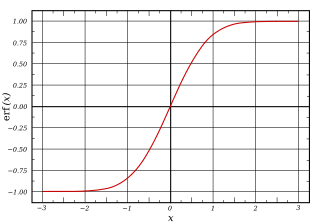
In general, a sigmoid function is monotonic, and has a first derivative which is bell shaped. Conversely, the integral of any continuous, non-negative, bell-shaped function (with one local maximum and no local minimum, unless degenerate) will be sigmoidal. Thus the cumulative distribution functions for many common probability distributions are sigmoidal. One such example is the error function, which is related to the cumulative distribution function of a normal distribution; another is the arctan function, which is related to the cumulative distribution function of a Cauchy distribution.

A sigmoid function is constrained by a pair of horizontal asymptotes as $x\rightarrow \pm \infty$.

A sigmoid function is convex for values less than a particular point, and it is concave for values greater than that point: in many of the examples here, that point is 0.

Examples

Some sigmoid functions compared. In the drawing all functions are normalized in such a way that their slope at the origin is 1.

• Logistic function $$f(x)={\frac {1}{1+e^{-x}}}$$
• Hyperbolic tangent (shifted and scaled version of the logistic function, above) $$f(x)=\tanh x={\frac {e^{x}-e^{-x}}{e^{x}+e^{-x}}}$$
• Arctangent function $$f(x)=\arctan x$$
• Gudermannian function $$f(x)=\operatorname {gd} (x)=\int _{0}^{x}{\frac {dt}{\cosh t}}=2\arctan \left(\tanh \left({\frac {x}{2}}\right)\right)$$
• Error function $$f(x)=\operatorname {erf} (x)={\frac {2}{\sqrt {\pi }}}\int _{0}^{x}e^{-t^{2}}\,dt$$
• Generalised logistic function $$f(x)=\left(1+e^{-x}\right)^{-\alpha },\quad \alpha >0$$
• Smoothstep function $$f(x)={\begin{cases}{\displaystyle \left(\int _{0}^{1}\left(1-u^{2}\right)^{N}du\right)^{-1}\int _{0}^{x}\left(1-u^{2}\right)^{N}\ du},&|x|\leq 1\\\\\operatorname {sgn}(x)&|x|\geq 1\\\end{cases}}\quad N\in \mathbb {Z} \geq 1$$
• Some algebraic functions, for example $$f(x)={\frac {x}{\sqrt {1+x^{2}}}}$$
• and in a more general form $$f(x)={\frac {x}{\left(1+|x|^{k}\right)^{1/k}}}$$
• Up to shifts and scaling, many sigmoids are special cases of $$f(x)=\varphi (\varphi (x,\beta ),\alpha ),$$ where $$\varphi (x,\lambda )={\begin{cases}(1-\lambda x)^{1/\lambda }&\lambda \neq 0\\e^{-x}&\lambda =0\\\end{cases}}$$ is the inverse of the negative Box–Cox transformation, and $\alpha <1$ and $\beta <1$ are shape parameters.
• Smooth transition function normalized to (-1,1):

$${\begin{aligned}f(x)&={\begin{cases}{\displaystyle {\frac {2}{1+e^{-2m{\frac {x}{1-x^{2}}}}}}-1},&|x|<1\\\\\operatorname {sgn}(x)&|x|\geq 1\\\end{cases}}\\&={\begin{cases}{\displaystyle \tanh \left(m{\frac {x}{1-x^{2}}}\right)},&|x|<1\\\\\operatorname {sgn}(x)&|x|\geq 1\\\end{cases}}\end{aligned}}$$ using the hyperbolic tangent mentioned above. Here, $m$ is a free parameter encoding the slope at $x=0$, which must be greater than or equal to ${\sqrt {3}}$ because any smaller value will result in a function with multiple inflection points, which is therefore not a true sigmoid. This function is unusual because it actually attains the limiting values of -1 and 1 within a finite range, meaning that its value is constant at -1 for all $x\leq -1$ and at 1 for all $x\geq 1$. Nonetheless, it is smooth (infinitely differentiable, $C^{\infty }$) everywhere, including at $x=\pm 1$.

Applications

Inverted logistic S-curve to model the relation between wheat yield and soil salinity

Many natural processes, such as those of complex system learning curves, exhibit a progression from small beginnings that accelerates and approaches a climax over time. When a specific mathematical model is lacking, a sigmoid function is often used.

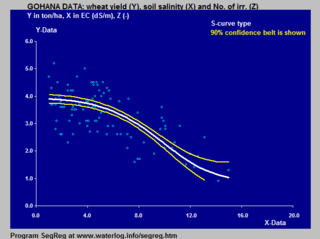
The van Genuchten–Gupta model is based on an inverted S-curve and applied to the response of crop yield to soil salinity.

Examples of the application of the logistic S-curve to the response of crop yield (wheat) to both the soil salinity and depth to water table in the soil are shown in modeling crop response in agriculture.

In artificial neural networks, sometimes non-smooth functions are used instead for efficiency; these are known as hard sigmoids.

In audio signal processing, sigmoid functions are used as waveshaper transfer functions to emulate the sound of analog circuitry clipping.

In biochemistry and pharmacology, the Hill and Hill–Langmuir equations are sigmoid functions.

In computer graphics and real-time rendering, some of the sigmoid functions are used to blend colors or geometry between two values, smoothly and without visible seams or discontinuities.

Titration curves between strong acids and strong bases have a sigmoid shape due to the logarithmic nature of the pH scale.

The logistic function can be calculated efficiently by utilizing type III Unums.

See also

• Step function – Linear combination of indicator functions of real intervals
• Sign function – Mathematical function returning -1, 0 or 1
• Heaviside step function – Indicator function of positive numbers
• Logistic regression – Statistical model for a binary dependent variable
• Logit – Function in statistics
• Softplus function – Type of activation functionPages displaying short descriptions of redirect targets
• Soboleva modified hyperbolic tangent – Mathematical activation function in data analysis
• Softmax function – Smooth approximation of one-hot arg max
• Swish function – Mathematical activation function in data analysis
• Weibull distribution – Continuous probability distribution
• Fermi–Dirac statistics – Statistical description for the behavior of fermions

Further reading

• Mitchell, Tom M. (1997). Machine Learning. WCB McGraw–Hill. ISBN 978-0-07-042807-2.. (NB. In particular see "Chapter 4: Artificial Neural Networks" (in particular pp. 96–97) where Mitchell uses the word "logistic function" and the "sigmoid function" synonymously – this function he also calls the "squashing function" – and the sigmoid (aka logistic) function is used to compress the outputs of the "neurons" in multi-layer neural nets.)
• Humphrys, Mark. "Continuous output, the sigmoid function". Archived from the original on 2022-07-14. Retrieved 2022-07-14. (NB. Properties of the sigmoid, including how it can shift along axes and how its domain may be transformed.)

External links

• "Fitting of logistic S-curves (sigmoids) to data using SegRegA". Archived from the original on 2022-07-14.

References

[edit]- ^ Han, Jun; Morag, Claudio (1995). "The influence of the sigmoid function parameters on the speed of backpropagation learning". In Mira, José; Sandoval, Francisco (eds.). From Natural to Artificial Neural Computation. Lecture Notes in Computer Science. Vol. 930. pp. 195–201. doi:10.1007/3-540-59497-3_175. ISBN 978-3-540-59497-0.
- ^ Ling, Yibei; He, Bin (December 1993). "Entropic analysis of biological growth models". IEEE Transactions on Biomedical Engineering. 40 (12): 1193–2000. doi:10.1109/10.250574. PMID 8125495.
- ^ Dunning, Andrew J.; Kensler, Jennifer; Coudeville, Laurent; Bailleux, Fabrice (2015-12-28). "Some extensions in continuous methods for immunological correlates of protection". BMC Medical Research Methodology. 15 (107): 107. doi:10.1186/s12874-015-0096-9. PMC 4692073. PMID 26707389.
- ^ "grex --- Growth-curve Explorer". GitHub. 2022-07-09. Archived from the original on 2022-08-25. Retrieved 2022-08-25.
- ^ EpsilonDelta (2022-08-16). "Smooth Transition Function in One Dimension | Smooth Transition Function Series Part 1". 13:29/14:04 – via www.youtube.com.
- ^ Gibbs, Mark N.; Mackay, D. (November 2000). "Variational Gaussian process classifiers". IEEE Transactions on Neural Networks. 11 (6): 1458–1464. doi:10.1109/72.883477. PMID 18249869. S2CID 14456885.
- ^ Smith, Julius O. (2010). Physical Audio Signal Processing (2010 ed.). W3K Publishing. ISBN 978-0-9745607-2-4. Archived from the original on 2022-07-14. Retrieved 2020-03-28.
- ^ Gustafson, John L.; Yonemoto, Isaac (2017-06-12). "Beating Floating Point at its Own Game: Posit Arithmetic" (PDF). Archived (PDF) from the original on 2022-07-14. Retrieved 2019-12-28.